Using table calculations to build an amortisation table
How to Build an AmortiSation Table
After working closely with a client in the banking industry, I saw some potential in how Tableau could be used as a simple loan simulator that would give you insight into your instalment payments, given an interest rate, loan duration and the borrowed amount.
First things first, back to basics.
It is almost a universal truth that borrowing money from institutions costs money. Repaying the principal and interest amount is usually done through instalments over an agreed upon time range. Regardless of whether you are a borrower or a lender, keeping track of the outstanding balance at any point in time is important.
A default amortisation table not only gives you a quick overview on the amount that is still owed, but also gives you insight into how much of your instalment is allocated to paying off the principal and interest. Typically, the longer the loan duration, the smaller your monthly instalments, but the higher your interest costs over the entire loan duration.
Building blocks of a simple loan simulator
As Leonardo Da Vinci said: ‘Simplicity is the ultimate sophistication’. The only data you will need is a calendar that contains the right granularity for the type of instalment that is going to be simulated. All the other information will be loaded as parameters in Tableau.
Setting up the amortiSation logic in Tableau
This particular example is assuming fixed-rate loans with monthly instalments.
Tableau Workbook with these examples can be downloaded here.
Data file used within Tableau Workbook can be downloaded here.
-
Loan amount
-
Loan duration (in months, for this particular example)
-
Interest rate (annual, for this particular example)
-
Monthly Interest Rate
-
Annual Interest Rate/12
-
# of payments to be made
-
WINDOW_MAX(INDEX())-INDEX()
-
For every row in the amortisation table, this field calculates how many payments still need to be made. Make sure you calculate this using Table Down.
-
Outstanding Principal
-
((1-(1+[Monthly Interest Rate])^(- [# of payments made])) * [Total Monthly Payment]) / [Monthly Interest Rate]
-
The outstanding principal in period x is a result of outstanding principal in period x-1 minus the principal in period x .
-
Total Monthly Payment
-
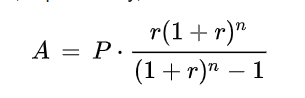
[Loan]*((([Monthly Interest Rate]*((1+[Monthly Interest Rate])^[Loan Duration in Months])))/(((1+[Monthly Interest Rate])^[Loan Duration in Months])-1))
-
This calculated field is using the standard amortisation formula.
-
A = monthly payment
-
P = principal
-
R = monthly interest rate
-
n = number of payments
-
The amount of this recurring payment will be fixed throughout the entire life of duration. However, the share designated to the interest and principal repayment will change over time.
-
Due Interest
-
IFNULL(LOOKUP([Outstanding Principal], -1), [Loan])*[Monthly Interest Rate]
-
The interest in period x is calculated against the outstanding principal in period x-1. Consequently, as the outstanding principal diminishes over time, the monthly instalment designated to paying off interest will also reduce, whilst the principal’s share will increase to keep the total monthly payment in balance.
-
Due Principal
-
[Total Monthly Payment]- [Due Interest]
Spice up your loan calculator!
Some ideas for more advanced simulations;
-
Instead of using fixed interest rates, make the simulation more realistic by using compound interest rates
-
Make your simulations more widely applicable by adding in a parameter that allows you to simulate monthly vs quarterly repayments
-
...
- Yun